Snowflake's REDUCE Function to Glean Insights from SEC Filing Data

 Summary

• What is the REDUCE Higher-order Function?
• Learn the JSON structure of the SEC company filing from an example.
• What fiscal end periods are represented in the JSON document?
• Answer the question using the REDUCE higher-order function in Snowflake.

What is the REDUCE Higher-order Function?

Recently, Snowflake made REDUCE Higher-order function generally available. This function adds another powerful, easy-to-use tool to your toolkit to process arrays. The REDUCE function allows you to accumulate values across an array into a single value. It takes an array as input, an initial accumulator value, and a Lambda expression that defines the logic for processing each array element.

REDUCE( <array> , <init> , <lambda_expression> ) 

The JSON Structure of the SEC Filing

My goal is to understand the cash carried by Kimberly-Clark Corporation in its balance sheet. The company is known for its products, such as Huggies and Cottonelle. I want to list all the fiscal end dates in the data. There can be inconsistencies in the data filed with the SEC, especially concerning the fiscal periods represented, so knowing what fiscal periods are in the data can be invaluable. Also, the SEC filing may have repeated data. This is because investors wish to compare current results with past results, so a Q2 report should include Q1 and Q2 data from the previous year. So, the SEC filing would have repetitions.

Note: You can learn about my External Table structure here. In my LinkedIn profile, you can read a series of blogs about my setup to query SEC filings.

Here's the JSON structure we will use in the REDUCE function:

{ 
"cik": 55785, 
"description": "Amount of currency on hand as well 

as demand deposits with banks or financial institutions. 

Includes other kinds of accounts that have the general characteristics of 

demand deposits.", 
"entityName": "KIMBERLY-CLARK CORPORATION", 
"label": "Cash and Cash Equivalents, at Carrying Value", 
"tag": "CashAndCashEquivalentsAtCarryingValue", 
"taxonomy": "us-gaap", 
"units":  { 
"USD": [
                  { 
                    "accn": "0001193125-10-038621", 
                    "end": "2006-12-31", 
                    "filed": "2010-02-24", 
                    "form": "10-K", 
                    "fp": "FY", 
                    "frame": "CY2006Q4I", 
                    "fy": 2009, 
                    "val": 361000000 
                  }, 
                  {
                    "accn": "0000055785-09-000026", 
                    "end": "2007-12-31", 
                    "filed": "2009-08-07", 
                    "form": "10-Q", 
                    "fp": "Q2", 
                    "fy": 2009, 
                    "val": 473000000
                  }
               ]
                }
}

What fiscal end periods are represented in the JSON document?

I have created an external table called CONS_STAPLES_CASH_AND_CASH_EQUIVALENTS. For the REDUCE function, the input is the path to the array:

Path to the Array Elements:

VALUE:"units":"USD" 

I wish to get a concatenated string of all the fiscal end periods represented in the JSON document. This is represented by the "end" key. This is represented in the init parameter as ''. Finally, in the Lambda Expression, the arg1 argument is the accumulator, and the arg2 argument is the current element being processed in the array.

Lambda Expression and the Query:

(arg1, arg2) -> arg1 || ' ' || arg2:"end" || ', '

SELECT 
            TICKER_SYMBOL, 
            VALUE, 
            REDUCE(VALUE:"units":"USD", '',  (arg1, arg2) -> arg1 || ' ' || arg2:"end" || ', ')           
                                                                                             FISCAL_PERIOD_END_DATES 
FROM 
            CONS_STAPLES_CASH_AND_CASH_EQUIVALENTS_ET;

When I execute the query, the REDUCE function retrieves the value for the "end" key, concatenates it to the accumulator, and returns it (Exhibit 1). The screenshot shows that for Kimberly-Clark Corp (KMB), the JSON has data from the fiscal period ending 2006-12-31. But for Target (TGT), the data in the JSON is from 2016-01-30.

Exhibit 1: The Fiscal Period End Date Returned by the REDUCE function.

Snowflake Snowsight

I can also tell that the SEC filing has duplicate data that I must handle in my query. For example, I can see that the 2007-12-31 is represented multiple times in the file I downloaded from the SEC (Exhibit 2).

Exhibit 2: Fiscal Period End Dates Accumulated By the REDUCE Higher-order Function.

SEC.GOV

I can quickly see the data in my JSON files downloaded from the SEC. I did not have to use a LATERAL FLATTEN to get at the data. The REDUCE function boosts my efficiency when I am dealing with JSON data. Try out Snowflake's REDUCE and other Higher-order functions; they will make you more productive.

Purchase Price Matters: Implementing Volume-Weighted Average Price (VWAP) in Snowflake

 Summary:

• A brief description of VWAP and its importance in trading and asset management.

• The process to calculate VWAP.

• An overview of the Snowflake features used to implement VWAP.

• The architecture of VWAP implementation in Snowflake.

• Code examples

• Examples of charting Microsoft's and Nestle's VWAP in Python.

What is VWAP?

Volume-weighted Average Price (VWAP) is a price signal that takes into account the trading volume. The logic behind the VWAP is simple: if investors think an asset is undervalued compared to its current price, they will purchase more of that asset. Investors use the VWAP as a benchmark price to make buying or selling decisions. If an asset is currently trading above the VWAP for the day, the trader may decide to sell or short an asset with the expectation that the asset would revert to the VWAP line, giving the trader a handsome profit. A trader may consider taking a long position if the asset's current price is below the VWAP.

A portfolio manager looking to acquire assets for her fund may use VWAP as the price to beat - a purchase price at or below VWAP would be considered reasonable. The portfolio manager would feel happy that she did not overpay for an asset.

Purchase Price Matters

The title of this article—Purchase Price Matters—comes from the excellent interview conducted by Nicolai Tangen (CEO of Norges Bank Investment Management) of Marc Rowan (CEO of Apollo Global Management, Inc.). Marc uses this phrase to state that every investment is a value investment. If you overpay for an asset, your investment returns will be lower - a simple yet profound thought. You can listen to the interview in the podcast - In Good Company With Nicolai Tangen. There are many amazing interviews in this podcast. These are three other episodes I would highly recommend:

• Vinod Khosla: Future Trends and the Power of the Improbable.

• Sal Khan - Personalized education, AI, and the drive to learn.

• Satya Nadella, Microsoft Chairman & CEO: AI, chip shortage, empathy, and poetry

VWAP Calculation

Investment firms may have their proprietary methodology for calculating VWAP. To implement VWAP in Snowflake, I have followed the method outlined in Investopedia, considering data availability and simplicity.

Here are the steps in this method:

• Take the average of high, low, and close prices for each period.

• If your VWAP period is 5 minutes, you will take the average of the high, low, and close for this period during the trading day. You arrive at the Typical Price for the asset.

  Typical Price (TP) = (High + Low + Close) / 3

• In my calculation, I only used the closing price for a period as my Typical Price.

• Next, multiply the Typical Price by the Trading Volume in this period.

Typical Price Volume (TPV) = Typical Price * Volume

• The VWAP is calculated by dividing the Typical Price Volume by the Volume. In this case, the VWAP for the first 5-minute time period would equal the Typical Price.

VWAP = Typical Price Volume / Volume

• The final step is to calculate the cumulative TPV over a period of time (for e.g. 60 minutes, a day, several days, or a year) and divide it by the sum of volume over the same period.

Cumulative VWAP = (TPV 1st 5-Min) + TPV 2nd 5-Min)/SUM(Vol 1st 5-Min + Vol 2nd 5-Min)

Data Provider

I used Polygon.IO as the data provider. In its free tier, Polygon provides a trade aggregates API that aggregates trades over 1-minute, 5-minutes, hours, days, weeks or months. I have used this data to demonstrate the VWAP implementation in Snowflake. The aggregates data is in the format:

{
  "adjusted": true,
  "next_url": "https://api.polygon.io/v2/aggs/ticker/AAPL/range/1/day/1578114000000/2020-01-10?cursor=bGltaXQ9MiZzb3J0PWFzYw",
  "queryCount": 1,
  "request_id": "6a7e466379af0a71039d60cc78e72282",
  "results": [
    {
      "c": 75.0875,
      "h": 75.15,
      "l": 73.7975,
      "n": 1,
      "o": 74.06,
      "t": 1577941200000,
      "v": 135647456,
      "vw": 74.6099
    },
  ],
  "resultsCount": 1,
  "status": "OK",
  "ticker": "AAPL"
}

VWAP Implementation on Snowflake

Before we get into the architecture, let's introduce some of the Snowflake features used to implement VWAP:

• Snowflake Storage Integration stores the identity and access information for the AWS S3 Bucket.

• A Snowflake Stage object identifies the location where the files are stored.

• Snowflake Snowpipe enables loading of data from files in batches. One can use a COPY statement in Snowpipe to automate the loading of file. An AWS S3 Bucket can be configured to notify Snowpipe of available files to load into Snowflake using AWS Simple Queue Service (SQS).

• The COPY INTO <table> SQL statement helps load data from files into an existing table.

• Snowflake Dynamic Tables offers a simple way to automate the transformation of data. You can easily create data pipelines using Dynamic Tables.

• The TIME_SLICE SQL function calculates the beginning or end of a "slice" of time.

• The Window functions are used to aggregate data over a period of time. I use this to calculate the cumulative VWAP. The Window functions are used to aggregate over a group of related rows, known as a partition. In our case the partion is the TICKER_SYMBOL - MSFT, AAPL, PEP, etc.

• Snowflake Pandas API allows you to run Pandas code in a distributed manner.

This is the architecture (Exhibit 1):

Exhibit 1: Volume-Weighted Average Price Architecture.

VWAP Implementation on Snowflake

• I use a Python app to access the Polygon API and store the JSON output in an AWS S3 Bucket.

• The AWS S3 Bucket is configured to notify Snowflake Snowpipe when a file lands in the Bucket.

• When Snowpipe receives the notification, its picks up the file from the Bucket and loads the raw JSON data into a table in Snowflake.

• At this point, a Dynamic Table, PARSE_STOCK_TRADES_DT, starts the process of transforming the JSON data by parsing the various keys.

• Another Dynamic Table, STOCK_TRADES_INTERMEDIATE_VWAP_DT, calculates the VWAP for various stocks over 20-minute time slices. In short, we take the 1-minute aggregate data from Polygon and calculate the VWAP for 20-minute slices.

• Finally, the last Dynamic Table, VWAP_STOCK_TRADES_DT, calculates the cumulative VWAP using a Window function to aggregate the price and volume data over all the previous rows and the current row.

• The final VWAP from the VWAP_STOCK_TRADES_DT can be presented in a dashboard as a chart.

The Snowflake Code Samples

Creating a Storage Integration

CREATE STORAGE INTEGRATION companystockprices_storage_int 
TYPE = EXTERNAL_STAGE STORAGE_PROVIDER = 'S3' 
ENABLED = TRUE 
STORAGE_AWS_ROLE_ARN = '<AWS  IAM Role ARN>' STORAGE_ALLOWED_LOCATIONS = ('*');

Create a Stage Object

CREATE STAGE COMPANY_STOCK_TRADES_STG 
URL = '<AWS S3 Bucket Path>' 
STORAGE_INTEGRATION = companystockprices_storage_int;

Create a Table to Store the JSON Trade Data

CREATE OR REPLACE TRANSIENT TABLE COMPANY_STOCK_TRADES_RAW 
( 
TICKER VARIANT, 
RESULTS VARIANT
);

Create a Snowpipe

CREATE OR REPLACE PIPE COMPANY_STOCK_TRADES_PIPE 
AUTO_INGEST = TRUE 
AS 
COPY INTO DEMODB.EQUITY_RESEARCH.COMPANY_STOCK_TRADES_RAW 

FROM @DEMODB.EQUITY_RESEARCH.COMPANY_STOCK_TRADES_STG 

MATCH_BY_COLUMN_NAME = CASE_INSENSITIVE 
FILE_FORMAT = (type = 'JSON' STRIP_OUTER_ARRAY = TRUE);

Create a Dynamic Table to Store the Parsed Data from the Raw Table

CREATE OR REPLACE TRANSIENT DYNAMIC TABLE PARSE_STOCK_TRADES_DT 
( 
TICKER_SYMBOL   VARCHAR, 
TRADE_TIME           TIMESTAMP_NTZ, 
TRADE_PRICE         NUMBER(20, 4), 
TRADE_VOLUME    NUMBER
) 
TARGET_LAG = DOWNSTREAM 
WAREHOUSE = DEMO_XSMALL_WH 
REFRESH_MODE = INCREMENTAL 
AS 
SELECT 
TICKER::VARCHAR TICKER_SYMBOL, 

TO_TIMESTAMP_NTZ(TO_NUMBER(trades.VALUE:"t"),3) TRADE_TIME, 

TO_NUMBER(trades.VALUE:"c",14, 4) 

TRADE_PRICE, TO_NUMBER(trades.VALUE:"v") TRADE_VOLUME 
FROM 
COMPANY_STOCK_TRADES_RAW CSTR, 
LATERAL FLATTEN (input => CSTR.RESULTS) TRADES 
ORDER BY TICKER_SYMBOL, TRADE_TIME;

Create a Dynamic Table to Calculate the Intermediate VWAP

CREATE OR REPLACE TRANSIENT DYNAMIC TABLE INTERMEDIATE_VWAP_STOCK_TRADES_DT 
( 
TRADE_TIME_SLICE                TIMESTAMP_NTZ, 
TICKER_SYMBOL                   VARCHAR, 
SUM_PRICE                       NUMBER(20, 4), 
SUM_VOLUME                      NUMBER, 
INTERMEDIATE_SUM_PRICE_VOLUME   NUMBER(20, 4), 
INTERMEDIATE_VWAP               NUMBER(20, 4)
) 
TARGET_LAG = DOWNSTREAM 
WAREHOUSE = DEMO_XSMALL_WH 
REFRESH_MODE = INCREMENTAL 
AS 
SELECT 
TIME_SLICE(TRADE_TIME, 20, 'MINUTE') TRADE_TIME_SLICE, 

SUM(TRADE_PRICE)    SUM_PRICE,

SUM(TRADE_VOLUME)   SUM_VOLUME, 

SUM(TRADE_PRICE * TRADE_VOLUME) INTERMEDIATE_SUM_PRICE_VOLUME,
 
SUM(TRADE_PRICE * TRADE_VOLUME)/SUM(TRADE_VOLUME)  INTERMEDIATE_VWAP 

FROM  
PARSE_STOCK_TRADES_DT 
GROUP BY TICKER_SYMBOL, TRADE_TIME_SLICE
ORDER BY TICKER_SYMBOL, TRADE_TIME_SLICE; 

Create a Dynamic Table to Calculate the Cumulative VWAP

CREATE OR REPLACE TRANSIENT DYNAMIC TABLE VWAP_STOCK_TRADES_DT 
( 
TRADE_TIME_SLICE                    TIMESTAMP_NTZ, 
TICKER_SYMBOL                       VARCHAR, 
TICKER_SYMBOL_TRADE_TIME_SLICE      VARCHAR,  
CUMULATIVE_PRICE                    NUMBER(20,4), 
CUMULATIVE_VOLUME                   NUMBER, 
FINAL_VWAP                          NUMBER(20,4)
) 
TARGET_LAG = '30 minutes' 
WAREHOUSE = DEMO_XSMALL_WH 
REFRESH_MODE = INCREMENTAL 
AS 
SELECT 

TRADE_TIME_SLICE, 
TICKER_SYMBOL, 

(SUM(SUM_PRICE) OVER  (PARTITION BY TICKER_SYMBOL ORDER BY TRADE_TIME_SLICE ASC ROWS 

BETWEEN UNBOUNDED PRECEDING AND CURRENT ROW)) CUMULATIVE_PRICE, 

(SUM(SUM_VOLUME) OVER (PARTITION BY TICKER_SYMBOL ORDER BY TRADE_TIME_SLICE ASC ROWS 

BETWEEN UNBOUNDED PRECEDING AND CURRENT ROW)) CUMULATIVE_VOLUME,

(SUM(INTERMEDIATE_SUM_PRICE_VOLUME) OVER (PARTITION BY TICKER_SYMBOL 

ORDER BY TRADE_TIME_SLICE ASC ROWS BETWEEN UNBOUNDED PRECEDING AND CURRENT ROW))

/(SUM(SUM_VOLUME) OVER (PARTITION BY TICKER_SYMBOL ORDER BY TRADE_TIME_SLICE ASC ROWS 

BETWEEN UNBOUNDED PRECEDING AND CURRENT ROW)) FINAL_VWAP 

FROM 
INTERMEDIATE_VWAP_STOCK_TRADES_DT 

ORDER BY TICKER_SYMBOL, TRADE_TIME_SLICE ASC;

You can visualize the data pipeline in Snowflake Snowsight (Exhibit 2). The active Dynamic Tables are shown with the dark blue arrows.

Exhibit 2: Data Pipeline Graph in Snowsight.

Data Pipeline Visualized in Snowsight

Charting Intermediate and Cumulative VWAP in Python

In Snowflake Notebook, you can easily create a session object using get_active_session()

import streamlit as st 
import matplotlib.pyplot as plt 
import seaborn as sns

# Snowpark Pandas API. 
# We are loading all the data in the Snowflake Pandas Data Frame.

import modin.pandas as spd 

# Import the Snowpark pandas plugin for modin 
import snowflake.snowpark.modin.plugin 

from snowflake.snowpark.context import get_active_session
 # Create a snowpark session 
session = get_active_session()

# Name of the sample database and the schema to be used 

SOURCE_DATA_PATH = "DEMODB.EQUITY_RESEARCH" 

Query the intermediate VWAP values from the INTERMEDIATE_VWAP_STOCK_TRADES_DT

# Query the Intermediate VWAP Dynamic Table.

intermediate_VWAP_df = spd.read_snowflake(f"{SOURCE_DATA_PATH}

                .INTERMEDIATE_VWAP_STOCK_TRADES_DT")

                .sort_values(["TICKER_SYMBOL","TRADE_TIME_SLICE"], ascending = True) 

# Filter for the MSFT Values in the Pandas Data Frame.

filtered_intermediate_VWAP_df = intermediate_VWAP_df

                        .where(intermediate_VWAP_df['TICKER_SYMBOL'] == 'MSFT') 

# Remove all the NONE values from the Pandas Data Frame.

filtered_intermediate_VWAP_df = filtered_intermediate_VWAP_df.dropna()

Query the cumulative VWAP from the VWAP_STOCK_TRADES_DT

# Query the Cumulative VWAP Table 

final_VWAP_df = spd.read_snowflake(f"{SOURCE_DATA_PATH}.VWAP_STOCK_TRADES_DT")

# Filter for the MSFT values in the Pandas Data Frame.

filtered_final_VWAP_df = final_VWAP_df.where(final_VWAP_df['TICKER_SYMBOL'] == 'MSFT') 

# Remove all the NONE values from the Pandas Data Frame.

filtered_final_VWAP_df = filtered_final_VWAP_df.dropna()

Merge the intermediate VWAP and the Cumulative VWAP to use in a Python chart.

# Merge the Intermediate VWAP and Cumulative VWAP

spd_intermediate_and_final_vwap_df = filtered_intermediate_VWAP_df.merge(filtered_final_VWAP_df,
                                            left_on='TICKER_SYMBOL_TRADE_TIME_SLICE', 
                                            right_on='TICKER_SYMBOL_TRADE_TIME_SLICE', 
                                            how='left')

Use the merged the Snowflake Pandas Data Frame to plot the chart.

data = {  
'TRADE_TIME_SLICE_x': spd_intermediate_and_final_vwap_df['TRADE_TIME_SLICE_x'], 

'INTERMEDIATE_VWAP': spd_intermediate_and_final_vwap_df['INTERMEDIATE_VWAP'], 

'FINALVWAP': spd_intermediate_and_final_vwap_df['FINAL_VWAP']
} 

df = spd.DataFrame(data)
 
# Create the plot 
plt.figure(figsize=(15, 6)) 

plt.plot(df['TRADE_TIME_SLICE_x'], df['INTERMEDIATE_VWAP'], label='INTERMEDIATE_VWAP') 

plt.plot(df['TRADE_TIME_SLICE_x'], df['FINAL_VWAP'], label='FINAL_VWAP') 

# Add title, labels, and legend 
plt.title('Microsoft Volume Weighted Average Price (VWAP)') 

plt.xlabel('TRADE') plt.ylabel('VWAP') plt.legend() # Show the plot plt.show()

I merged the intermediate VWAP (20-Minute Time Slice) and the cumulative VWAP (From Feb 2023) and plotted it in a chart in Snowflake Notebook using Python. Here's how it looks:

We can see from the chart (Exhibit 3) that Micrsoft is currently trading (Intermediate VWAP - blue line) well above its cumulative VWAP line (yellow line). Microsoft is benefitting from the AI-led demand for its products and services mixed with the euphoria and promise of more gains to come from AI-related product releases.

Exhibit 3: Microsoft's Intermediate VWAP (20-Minute Window) and Cumulative VWAP (Since Feb 2023)

Microsoft's Intermediate VWAP (20-Minute Window) and Cumulative VWAP (Since Feb 2023)

On the other end of the spectrum is Nestle. The company is having a no good, very bad year since October 2023. Its intermediate VWAP (20-Minute Time Slice) has dropped well below its cumulative VWAP (Exhibit 4). Nestle has suffered from sky rocketing prices for cocoa and coffee that has pressured its margins. This is Nestle, one of the most iconic brands with a multitude of well-known products and sales in over a 100 countries, it's in pretty bad shape today, but they should recover in the coming years.

Exhibit 4: Nestle Intermediate VWAP (20-Minute Time Slice) and Cumulative VWAP (Since Feb 2023).

Nestle Intermediate VWAP (20-Minute Time Slice) and Cumulative VWAP (Since Feb 2023).

In just a couple of hours you can ingest raw market data into Snowflake and transform it into signals such as Volume-Weighted Average Price (VWAP).

The Costco Paradox

What can we learn from the success of Costco?

Summary:

• An analysis of Costco and Walmart's revenue growth over the past eight years.
• A look at the gross margins of these two retailers.
• An analysis of the inventory costs of these retailers.

Costco (COST) is one of the most successful retailers in the world. It has a loyal customer base, its employees are among the highest paid in the retail sector, and that leads to lower employee turnover, and it has a very generous return policy, furthering its customer loyalty. The company presents multiple paradoxes. Here are just a few:

• How is Costco, with such low gross margins, not only still in business but thriving in the highly competitive retail sector?
• How does Costco succeed in the internet era when its e-commerce strategy is an afterthought?
• How does a retailer who pays and treats employees so well, but still manages to deliver superior shareholder returns?

Each retail company is unique in its own way. In many ways, uniquesness is a required feature for retailers. If a retailer is unable to distinguish themselves from the competition, they will not last long. Even among a crowded field of retailers, Costco and Trader Joe's standout. About 80% of products Trader Joe's sells is private label. In comparison, the U.S., with companies with strong brands and billions in marketing budgets, has seen only a 20% penetration by private label brands. Other retailers are yet to replicate Trader Joe's success in private label. Costco, for its part, does well with its Kirkland private label brand, selling many products under this label. Since this is an article about Costco, let's turn our attention to this great American company.

Costco Wholesale is unique in it own way. The way company operates and caters to its customers is a study in human psychology. Over 90% of its members renew each year. The store delivers a treasure hunt experience because you never know what you will find in each aisle. The aisles remain unmarked yet customers aren't frustrated. Over the years Costco has trained its customers to have a mental map of where they could typically find essential items. For example, paper towels and cleaning supplies are typically found at the back of the store.

Costco's executive memberships cost $130 annually yet, over 35 million out of their 76 million total members chose this level rather than pay $65 for the Gold Star membership (Exhibit 1). People perceive much value received from their executive membership. Members know Costco will never overcharge them. The company prides itself in keeping its mark-up 14%-15% above its costs, an extremely low number for a retailer. Costco pays a 2% reward on purchases to their executive members which many feel will help them recoup their membership cost. This reward eats into their already tiny margins, but Costco chose loyal customer base over higher margins. I am willing to theorize that consumers, if given a choice to pick between Amazon Prime and Costco memberships, will overwhelmingly pick Costco.

Exhibit 1: Costco Q4 FY 2024 Membership Numbers and Renewal Rate.

Source: Costco Investor Relations.

What are Costco's Revenue and Growth Rate?

Since 2008, Costco has increased its revenue by 3.5x, from $72 billion to $254 billion in 2024 (Exhibit 2). During the same period, Walmart (WMT), a much larger company, increased its revenue by 1.7x, from $377 billion in 2008 to $648 billion in 2024 (Exhibit 3). Just when people think that the market is saturated with Costco Warehouses, it finds new locations and customers. It has been expanding in China for years, although this comes with a side of geopolitical risk.

Exhibit 2: Costco Wholesale Revenue (2008 - 2024)

SEC.GOV, Snowflake Snowsight

Exhibit 3: Walmart Revenue (2008 - 2024)

SEC.GOV

Costco's revenue grew at an average annual rate of 8.2% between 2008 and 2024. But, if you remove the pandemic-era binge shopping between 2020 and 2022, the growth rate was 6.9%, still an impressive number. Walmart averaged a revenue growth rate of 3.4% between 2008 and 2024, including the pandemic years.

Exhibit 4: Costco's Annual Revenue Growth Rate.

Snowflake Cortex Analyst, Excel

Exhibit 5: Walmart's Annual Revenue Growth Rate.

Snowflake Cortex Analyst, Excel

What are Costco's Gross Margins?

Costco has one of the lowest gross margins among retailers. Costco's gross margin in 2024 was 12.6% compared to 27.6% for Target (TGT), and 24.3% for Walmart. This is by design and may be their secret weapon. A company has to have strict financial discipline when it starts off with such low gross margins. Richard Galanti, the former CFO of Costco, was adept at managing costs. For the most part he was Costco's voice in Wall Street, presenting at the company quarterly earnings calls. Richard managed Costco's investments well, from inventory costs, new store openings, and e-commerce expenditures.

Costco's gross margins are well below that of Target and Walmart.

Exhibit 6: Gross Margins of Target, Walmart, and Costco.

SEC.GOV

How does Costco's Inventory Costs Compare with Walmart's and Target's?

Inventory is one of the largest costs for any retailer. When managed efficiently, inventory can boost operating cashflows and margins. When managed poorly, inventory can lead to losses or worse, bankruptcy.

Days of Sales in Inventory ( DSI) is a good metric to measure the efficiency of a company's inventory costs. This ratio indicates the average time in days it takes a company to sell its inventory. This metric also helps comparing inventory management efficiency across companies in a sector. Costco carries the least amount of inventory as possible on its balance sheet. It also helps that its loyal customer base regularly shops at the stores and helps clean out their inventory quickly.

Costco manages its inventory very efficiently compared to Walmart or Target. Costco manages to turnover its inventory every 31 days compared to nearly 41 days for Walmart and 56 days for Target (Exhibit 7 & 8). I have used ending inventory for each fiscal year in this calculation. When the ending inventory is used to calculate the days sales in inventory, the average number of days for Costco to turnover its inventory is 31.2 days.

Exhibit 7: Days Sales In Inventory For Walmart, Target, Costco.

Snowflake Snowsight

Exhibit 8: Costco Revenue, COGS, Gross Margin, and Days Sales in Inventory (Using Ending Inventory)

Snowflake, Excel

In Exhibit 9, I have used the average inventory to calculate the days sales in inventory. The average number of days it takes Costco to turnver its inventory in this case is 29.9 days.

Exhibit 9: Costco Revenue, COGS, Gross Margin, and Days Sales in Inventory (Using Average Inventory)

Snowflake, Excel.

Costco teaches us that margins are just a number. How you manage that efficiently while focusing on delivering value to the customer is what makes or breaks a company. Costco focus on keeping costs low for their customers helps it sell more stuff faster reducing its inventory costs and giving it enormous clout over its suppliers.

Finally, I have used Snowflake Data Cloud for almost all of my analysis. Snowflake platform is easy to use to gain business insights. I have shown you example of that here.

Disclosures: I am a Sales Engineer at Snowflake. You can reach me here. All opinions in this blog post are solely mine and do not reflect Snowflake's views. I am not a Registered Investment Advisor, and any discussion on securities or investments is not an inducement to make a particular investment.

Impact of GenAI on R&D Expenditure

 Summary:

• Describe the AI money flow using an illustration.
• How much do Adobe, Salesforce, and others spend on Research and Development (R&D)?
• How has the R&D expense changed over time?
• What can we infer about the impact of GenAI on R&D expenses?

In this post, we examined Microsoft's capital expenditures (capex) as a proxy for the billions of dollars hyper-scaler cloud providers are investing in AI. Who is consuming this capex? We will answer this fundamental question in this post. Most people may already know the answer to this question. Cloud providers are packaging Nvidia GPUs into various IaaS services, offering them to companies such as Adobe, ServiceNow, Salesforce, and every other company in every industry experimenting with GenAI. These companies' investments in AI show up in research and development expenditures in the income statement.

The AI Money Flow

Here's how the investments in AI flows through various companies. Let's look at each step.

Source: Prasanna Rajagopal

1. Nvidia designs the GPUs.

2. Taiwan Semiconductor Manufacturing Company (TSMC) brings Nvidia's dreams to the market.

3. Dell, HP, and other server manufacturers, primarily based in Asia, buy these GPUs from Nvidia and package them into servers. The cost of the GPUs is included in the server manufacturers' Cost of Goods Sold (COGS).

4. Cloud providers purchase these servers. The cost of these AI servers is included in the capital expenditures.

5. Companies worldwide purchase IaaS and PaaS services created by cloud providers to experiment with and create various AI products and services for their customers.

6. Github Copilot, Salesforce's Einstein AI, ServiceNow AI agent, Apple Intelligence, and other products are examples of GenAI in the marketplace.

7. Once a product is ready to be released, companies typically create a SaaS service and introduce their GenAI products to consumers and other companies across various industries.

8. Consumers and companies pay for the GenAI service. Many services currently have a free and paid tier. The free service may typically have some restrictions on product use.

Companies such as Apple, Delta Airlines or Expedia build Chatbots, which they hope would help increase revenue, reduce the cost of serving their customers and thus boost their profit margins. But, most companies bringing GenAI products to market will have to see cost reductions in their operations soon or generate a profitable revenue stream.

Note about #2:

By now, most people are familiar with Jensen Huang, the unassuming, charismatic Nvidia founder. Most people probably have never heard of Morris Chang - the unassuming, spotlight-shunning, nonagenarian Taiwan Semiconductor Manufacturing Company (TSMC) founder. Here are a couple of articles to learn more about him:

• The Chip Titan Whose Life’s Work Is at the Center of a Tech Cold War

• He Turned 55. Then He Started the World’s Most Important Company.

Note about #5:

The cloud providers themselves are massive users of the GPUs they purchase. Internal product teams at Amazon and Microsoft are experimenting with and creating new GenAI products. These product development expenses appear as research and development (R&D) expenses. So, in addition to spending billions on capital expenditure, Amazon, Microsoft, and Google are racing to create new genAI products and, in turn, invest billions more in R&D.

Companies like Adobe, Apple, ServiceNow, Salesforce, and others are investing in GenAI R&D to create new products. Since Adobe, ServiceNow, and others do not buy the GPUs directly and maintain, for the most part, their own data centers, they rely on the cloud providers for their GPU and include the cost of buying those services in R&D. In this post, we will examine how those R&D expenses have changed for these companies with the advent of GenAI.

Note about #7:

When a product is released to the market by the R&D teams, the responsibility of maintaining the service is turned over to the Cloud Operations and Support teams at Adobe, Salesforce, ServiceNow, and others. The cost of providing these services to customers and the associated GPU use is included in the cost of goods sold (COGS).

Research and Development Spending By Companies

Apple's R&D Spending

Apple is one of the largest companies on the planet in terms of revenue, profits, and market value. They have also been slow to announce AI services, only recently announcing Apple Intelligence. Apple is a big R&D spender with one of the largest R&D budgets in the world. Apple spent nearly $30 billion on R&D in 2023.

Chart: Apple's Annual R&D Expense (2007 - 2023)

(Chart Created Using Snowflake Snowsight)

Table: Apple's Annual R&D Spending

Queried in Snowflake, Table Formatted in Excel

Apple has increased its R&D budget by 38x since 2007. With the GenAI race just getting started, I do not see these massive expenses abating anytime soon. When you look at the chart below the R&D expense (yellow bar) compared to Revenue (blue bar) looks so tiny.

In fact, Apple only spent 7.8% of revenue on R&D. But, this is the company's highest spend in terms of dollar amounts and as a percent of revenue. The company increased its R&D spend by 114 basis points from 2022, adding over $3 billion to its R&D expense. Apple's motivation to release AI products and services may be behind this increase in R&D expense, especially at a time when its revenue declined from 2022 to 2023.

Chart: Apple's Annual R&D Spending Compared to Revenue

Created Using Snowflake Snowsight

Table: Apple's R&D Expense As a Percent of Revenue.

Queried in Snowflake, Table Formatted in Excel

Salesforce's R&D Expense

Let's look at R&D spending by Salesforce and how that's changed over time and feeling the pressure to invest in GenAI. Here's Salesforce's R&D expense compared to its annual revenues.

Chart: Salesforce's Revenue (blue bar) and R&D Expense (yellow bar)

Created Using Snowflake Snowsight

Table: Salesforce's Revenue and R&D Expense as a Percent of Revenue

Queried in Snowflake, Table Formatted in Excel

Salesforce has been spending above 14% of its revenue on R&D since 2017, well above Apple's expenditure in this category. Salesforce has probably decided that it is spending much on R&D already and only needs to reallocate, prioritize funds and teams to focus on GenAI projects.

Microsoft's R&D Expense

Microsoft is already spending plenty on capex. It is spending billions more on R&D. But as a percent of revenue, the company has not increased its spending. On dollar terms Microsoft has definitely increased it spending. Its R&D expense as a percent of revenue in 2024 was lower compared to 2023. But, in dollar terms the company increased its spending by over $2 billion.

Chart: Microsoft Revenue and R&D Expense

Created Using Snowflake Snowsight

Table: Microsoft's Revenue, R&D Expense, and R&D as a Percent of Revenue

Queried in Snowflake, Table Formatted in Excel

Companies that have were already spending well above 10% on R&D have probably prioritized the budgets with a focus on GenAI. Megatech companies such as Apple and Microsoft have increased their R&D expense by a few billion dollars. These fresh dollars are mostly likely focused on creating new AI products and services.

Disclosures: I am a Sales Engineer at Snowflake. All opinions in this blog post are solely mine and do not reflect Snowflake's views. I am not a Registered Investment Advisor, and any discussion on securities or investments is not an inducement to make a particular investment.

Paccar: Peak Demand For Trucks

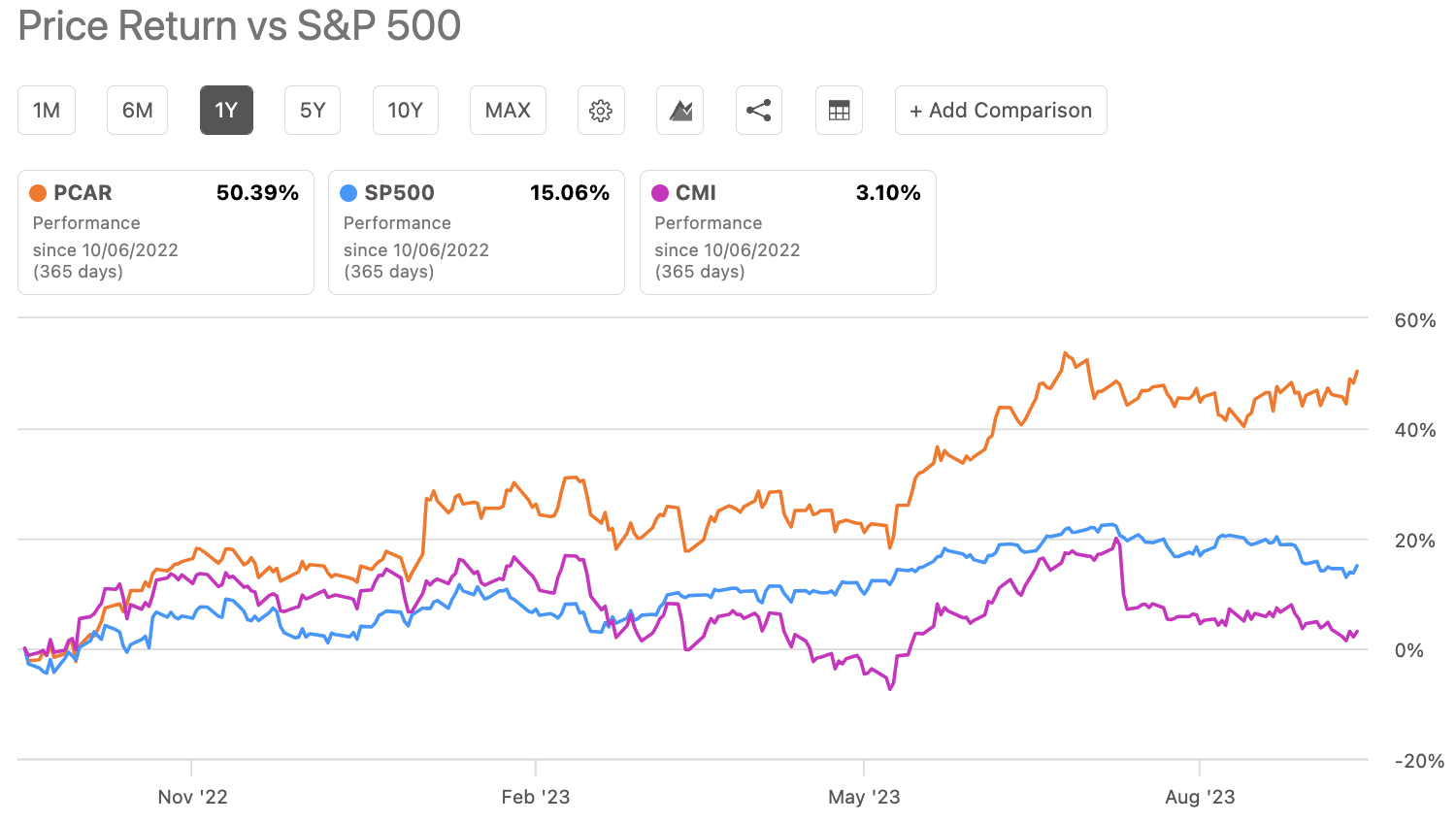
 Paccar (PCAR) produced 185,900 trucks in 2022 and is on track for another record year in 2023. The company has experienced good revenue growth in 2021 and 2022. The company has experienced stellar gross and operating margins over the past few years. The company registered a 16% gross and 13% operating margin in 2022. The current fiscal year, 2023, may bring even more good news on the margin front. The company registered a 20% gross and 17% operating margin in its March 2023 quarter and maintained its 17% operating margin in June 2023. 

Unfortunately, the demand for trucks may have peaked, given high-interest rates, high inflation, and waning consumer demand. Some of the strength in the truck market was due to the stimulus and subsidies provided by the U.S. Federal Government that bolstered infrastructure spending and brought about a manufacturing renaissance in this country. Although the bills passed by Congress in 2022 have more spending left for a few more years, the weakening consumer and lack of demand in the real estate sector may counteract the spending by the Federal Government. Fiscal year 2023 may be as good as it gets for Paccar. The stock has performed well over the past year, and its dividend yield has fallen. Dividend income seekers may have to wait for a much higher dividend before buying the stock. Treasury rates have increased enough that bonds offer an attractive alternative for investors waiting for a higher yield. Due to these reasons, I rate it a hold.

Exceptional performance of Paccar.

Paccar has performed exceptionally well over the past year, gaining 50% (Exhibit 1). The stock has handily outperformed the S&P 500, which has returned 15% over the past year. Cummins (CMI) gained just 3% over the past year. Year-to-date, the stock has gained 33% compared to the 12% return of the S&P 500 Index (SP500). The Vanguard Industrials Index Fund ETF (VIS) has had a great year, with a return of 16% over the past year. The industrial sector has benefitted from the stimulus and subsidy spending by the U.S. Federal Government. Although more subsidy spending is left in the coming years under the bill authorized by Congress in 2022, a combination of high interest rates and a slowing global economy may cap any upside in this stock.

Exhibit 1: 

Performance of Paccar, S&P 500, and Cummins (Seeking Alpha)

Fully valued

Although the stock, trading at a forward GAAP PE of 11.4x, looks undervalued compared to its five-year average of 14.4x, given the economic environment and the rate increase, this lower valuation may be deserved. The Vanguard Industrial Index ETF (VIS) may be overvalued, trading at a weighted average PE of 20x and a price/book ratio of 4x. The EV/EBITDA multiple may better assess the company’s valuation. The stock trades at a 10.2x forward EV/EBITDA multiple compared to the sector median of 10.7x. This indicates the stock may be fully valued. Cummins (CMI), a Paccar peer, looks undervalued, trading at a 7.8x forward EV/EBITDA multiple.

Dividends, buybacks, and debt.

Given the stock's performance over the past year, the yield has dropped to 1.2%. The Vanguard Industrials ETF offers a yield of 1.4%, and the Vanguard S&P 500 Index ETF yields 1.58%. The payout ratio is 12%, a rather conservative number. But, given the cyclical nature of the truck business, Paccar may be suitable to be cautious with its payout. A low payout may also free up cash for stock repurchases. The company paid $483 million in total dividend payments over the trailing twelve months. The company has grown its dividend annually at the pace of 7.5%, compared to 6.8% for the sector, over the past five years.

Paccar has spent $828 million in share buybacks over the past decade. But, the company has issued over $300 million in stock over the past decade, blunting the share buybacks' effects. The diluted share count is reduced from 532.8 million in 2013 to 524.1 million over the trailing twelve months, just 8.7 million. Using this share count reduction, the average price paid for the buybacks is $95 compared to its current price of $86.

The company generated $5.4 billion in EBITDA during the trailing twelve months. Paccar generated $3.5 billion in operating cash and $2.37 billion in free cash flow. This free cash flow number is derived by deducting the company’s capital expenditures from its operating cash. These numbers are good, but investors should remember that 2022 was one of the strongest years for truck demand globally, and 2023 is shaping to be another good year. I am concerned these good times, and any demand reduction could dent its cash flows. Also, the company generates a lot of revenue from its financing division. If the economy slows further and demand wanes, it could increase bad loans and decrease the demand for new loans, as the U.S. Treasury rates have increased to their highest levels in over a decade.

Paccar has performed exceptionally well over the past decade, returning 237% on a total return basis compared to the 210% return of the S&P 500 Index. But, weakening consumers coupled with high rates may put a substantial dent in demand across the various sectors of the economy. The stock’s performance has been impressive, and the industrial sector has been strong over the past year. Most of this strength may be attributed to the various bills passed by the U.S. Congress that have billions of dollars in outlays for renewable energy, electric vehicles, infrastructure modernization, and efforts to re-shore manufacturing and build semiconductor plants. Investors should be concerned that most of the demand across the industrial sector and Paccar is driven not by consumer organic demand but by the government's industrial policy. Paccar’s strength may not last, and it may be best for investors to wait for a much lower entry point.

The Industrials Sector is on a Tear

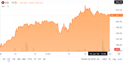
 The Vanguard Industrials Index ETF (VIS) touched a 52-week high of $202.86 on Friday, June 16 (Exhibit 1).  

Exhibit 1:

Vanguard Industrial Index ETF (VIS) 5-Day Performance
Source: Seeking Alpha

The top performer in this ETF was Vertiv Holdings, returning 133% over the past year (as of June 16, 2023). The company describes itself as follows:

"Vertiv is a global leader in the design, manufacturing and servicing of critical digital infrastructure for data centers, communication networks, and commercial and industrial environments. Our customers operate in some of the world's most critical and growing industries, including cloud services, financial services, healthcare, transportation, manufacturing, energy, education, government, social media, and retail." (Source: SEC.GOV)

This renewed interest in data centers is not surprising, given the popularity of artificial intelligence (AI) and the investments in new applications powered by AI. 

In the Q1 2023 Earnings call, Vertiv's management said the following about AI:

"We are distinctly seeing the first signs of the AI investment cycle in our pipelines and orders. Vertiv is uniquely positioned to win here, given our market leadership and deep domain expertise in areas like thermal management and controls, which are vital to support the complexity of future AI infrastructures." (Source: Seeking Alpha)

"Let me go back to the investments in AI. You may have heard it as generally characterized as the next infrastructure arms race, Vertiv benefits from this race and is an agnostic partner of choice to the risk participants. The acceleration in investment in AI will turn into a net infrastructure capacity demand acceleration, and this starts to be visible in our pipeline. AI applications’ demand and net capacity increase in the industry, higher power density, a gradual migration to an air and liquid hybrid cooling environment and a transition to liquid-ready facility designed." (Source: Seeking Alpha)

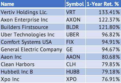
 Here's the list of the top 10 performers in the Vanguard Industrials Index ETF over the past year (Exhibit 2).  

Exhibit 2:

Top 10 Performers in the Vanguard Industrials Index ETF
Source: Barchart.com, Data Provided by IEX Cloud

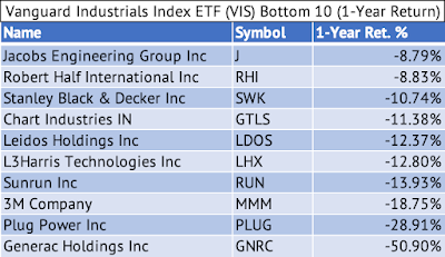
 Here's the list of the bottom 10 worst performers in the Industrials ETF over the past year (Exhibit 3):

Exhibit 3:

Bottom 10 Worst Performers in the Vanguard Industrials Index ETF
Source: Barchart.com, Data Provided by IEX Cloud