Corning's Volatility Compared to the Vanguard S&P 500 Index ETF

Here's the histogram of Corning's (GLW) monthly returns between June 2019 and October 2022 (Click on the image to see a larger version):

Exhibit: Corning's Monthly Returns Fell at or below 2.56% for the Majority of the Months

Data Provided by IEX Cloud, Author Calculations

There were 14 months between June 2019 and October 2022 when Corning's monthly returns were greater than 2.56%.  There were seven months when the monthly returns were greater than or equal to 11.5%.    

Corning's monthly returns have a high positive correlation of 0.66 with the monthly returns of the Vanguard S&P 500 Index ETF (VOO). 

Exhibit: The Vanguard S&P 500 Index and Corning Monthly Returns [June 2019 - October 2022]

Data Provided by IEX Cloud, Monthly Returns Calculated by the Author, Graph using RStudio 

A linear regression of the Vanguard S&P 500 Index ETF and Corning's monthly returns yields a beta of 1.03 for Corning. Corning's average monthly return will mirror the Vanguard S&P 500 Index ETF. Corning may not help diversify a portfolio and will not protect against the market's volatility.  

Here's the linear regression model:

> # Conduct the Linear Regression of the Monthly Returns Between $VOO and $GLW

> lmVOOGLW = lm(GLW_Monthly_Return~VOO_Monthly_Return, data = VOOandGLW)

> # Present the summary of the results from the linear regression

> summary(lmVOOGLW)

Call:

lm(formula = GLW_Monthly_Return ~ VOO_Monthly_Return, data = VOOandGLW)

Residuals:

      Min        1Q      Median     3Q       Max 

   -0.118363 -0.050928 -0.009998  0.041106  0.187435 

Coefficients:

                   Estimate     Std. Error   t value   Pr(>|t|)    

(Intercept)        -0.003778     0.010818    -0.349    0.729    

VOO_Monthly_Return  1.039148     0.188256     5.520    2.4e-06 ***

---

Signif. codes:  0 ‘***’ 0.001 ‘**’ 0.01 ‘*’ 0.05 ‘.’ 0.1 ‘ ’ 1

Residual standard error: 0.06823 on 39 degrees of freedom

Multiple R-squared:  0.4386, Adjusted R-squared:  0.4242 

F-statistic: 30.47 on 1 and 39 DF,  p-value: 2.403e-06

The coefficient for VOO_Monthly_Return [1.039148] is the beta for Corning.  The p-value is significant at a 95% confidence interval. The adjusted R-squared is 0.42, which means about 42% of Corning's average monthly return is explained by the Vanguard S&P 500 Index ETF returns.     

Monthly Return Comparison Between Cummins and Vanguard S&P 500 Index ETF

The following chart shows the Vanguard S&P 500 Index ETF (VOO) monthly returns on the x-axis and Cummins (CMI) on the y-axis. The regression line on the graph shows a steep slope, and the Pearson correlation value is 0.7. This value shows a very strong correlation between the monthly returns of the Vanguard S&P 500 Index ETF and Cummins. The p-value is significant at a 95% confidence interval. Cummins has returned 13.9% in the past year, while the Vanguard S&P 500 Index ETF has returned a -12.4%.  

Exhibit: Monthly Returns of Vanguard S&P 500 Index ETF and Cummins [June 2019 - October 2022]

   

The following command was used to create this graph:

> # Create a new Graph of $VOO and $CMI Monthly Returns as Percentages

> ggscatter(df1, x = 'VOO_Monthly_Return', y = 'CMI_Monthly_Return', 

+           add = "reg.line", conf.int = TRUE, 

+           cor.coef = TRUE, cor.method = "pearson",

+           xlab = "VOO ETF Monthly Returns (%)", ylab = "CMI Monthly +           Returns (%)")

A linear regression of the monthly returns of the Vanguard S&P 500 Index ETF and Cummins shows the beta (coefficient of Vanguard S&P 500 Index ETF) for Cummins' monthly returns compared to the Vanguard ETF. 

# Conduct the Linear Regression of the Monthly Returns Between $VOO and $CMI

lmVOOCMI = lm(CMI_Monthly_Return~VOO_Monthly_Return, data = VOOandCMI)

# Present the summary of the results from the linear regression

summary(lmVOOCMI)

Call:

lm(formula = CMI_Monthly_Return ~ VOO_Monthly_Return, data = VOOandCMI)

Residuals:

      Min        1Q    Median        3Q       Max 

-0.123268 -0.051037  0.004537  0.047062  0.115727 

Coefficients:

                   Estimate Std. Error t value Pr(>|t|)    

(Intercept)        0.005104   0.009226   0.553    0.583    

VOO_Monthly_Return 0.993327   0.160541   6.187 2.84e-07 ***

---

Signif. codes:  0 ‘***’ 0.001 ‘**’ 0.01 ‘*’ 0.05 ‘.’ 0.1 ‘ ’ 1

Residual standard error: 0.05819 on 39 degrees of freedom

Multiple R-squared:  0.4954, Adjusted R-squared:  0.4824 

F-statistic: 38.28 on 1 and 39 DF,  p-value: 2.845e-07

Cummins has a beta of 0.99 (nearly 1). Given this beta, Cummins, on average, moves in line with the S&P 500 Index. The adjusted R-squared value of 0.48 shows that about 48% of Cummins' monthly returns can be attributed to the returns of the S&P 500 Index. The p-value of 2.84e-07 shows that the regression analysis results are significant at the 95% confidence interval.

The average monthly return for Cummins between June 2019 and October 2022 was 1.49%. A one-sample t-test shows that the monthly return falls between -1.05% and 4.04%. But, the p-value of 0.99 is much higher than 0.05. This t-test may not be significant in the 95% confidence interval.        

#

# One Sample t-test of $CMI average monthly returns.

# 

# Step 1: 

# Copy Dataframe Column CMI_Monthly_Return into a List 

#

CMI_Monthly_Return_Col <- c(VOOandCMI['CMI_Monthly_Return'])

# CMI_Monthly_Return_Col is a list object, but needs to be numeric

# for qqnorm to work.  

#

typeof(CMI_Monthly_Return_Col)

# Convert List Object into a Column of doubles as as.numeric and unlist

#

y_CMI_Monthly_Return_Col <- as.numeric(unlist(CMI_Monthly_Return_Col))

typeof(y_CMI_Monthly_Return_Col)

# Let’s check if the data comes from a normal distribution 

# using a normal quantile-quantile plot.

# Source: https://cran.r-project.org/web/packages/distributions3/vignettes/one-sample-t-test.html

Exhibit: Check if Cummins' Monthly Returns are Normally Distributed before doing a t-test

#

qqnorm(y_CMI_Monthly_Return_Col)

qqline(y_CMI_Monthly_Return_Col)

# Conduct a t-test to see if the population mean is 1.49% [0.0149]

#

t.test(y_CMI_Monthly_Return_Col, mu = .0149)

One Sample t-test

data:  y_CMI_Monthly_Return_Col

t = 0.0045069, df = 40, p-value = 0.9964

alternative hypothesis: true mean is not equal to 0.0149

95 percent confidence interval:

 -0.01057188  0.04048574

sample estimates:

 mean of x 

0.01495693 

    

Volatility of Monthly Returns of Newell Brands Compared to the Vanguard S&P 500 Index ETF

The monthly returns of Newell Brands and the Vanguard S&P 500 ETF have a positive correlation of 0.44, as calculated using the Pearson method. The data used in this study is range from June 2019 to October 2022 (41 months of data). 

Newell Brands is a company that owns some very famous brands across multiple consumer and commercial product lines. 

Exhibit: The Brands Owned by Newell Brands

(Source: Newell Brands)

      

Here's the R command and the output from R-Studio

> # Calculate the Monthly Return Correlation between Newell Brands 

> # and Vanguard S&P 500 Index using the Pearson method 

> cor(VOOandNWL['NWL_Monthly_Return'], VOOandNWL['VOO_Monthly_Return'], method = c("person"))

                        VOO_Monthly_Return

NWL_Monthly_Return          0.4434957 

Here's the plot of the S&P 500 and the Newell Brands' monthly returns:

Exhibit: S&P 500 Index Monthly Returns VS. Newell Brands Monthly Returns

                       S&P 500 Index Monthly Returns against Newell Brands' Returns

                          (Source: Data Provided by IEX Cloud, Correlation and Graph on RStudio)

When the correlation is calculated for the months when the S&P 500 Index had positive returns, the correlation drops to 0.28. 

> # Calculate the Monthly Return Correlation between Newell Brands 

> # and Vanguard S&P 500 Index using the Pearson method

> # for only those months when the Vanguard S&P 500 Index ETF 

> # had positive returns.

> cor(VOOandNWLPositiveReturns['NWL_Monthly_Return'], VOOandNWLPositiveReturns['VOO_Monthly_Return'], method = c("person"))

                        VOO_Monthly_Return

NWL_Monthly_Return           0.284022

Here's the plot of the S&P 500 Index against Newell Brands' monthly returns for months when the S&P 500 index had a positive return. 

           Exhibit: S&P 500 Index Monthly Positive Returns VS. Newell Brands Monthly Returns

S&P 500 Index Monthly Returns (Positive Months) against Newell Brands' Returns

                          (Source: Data Provided by IEX Cloud, Correlation and Graph on RStudio)

The linear regression of the monthly returns of the S&P 500 index and Newell Brands is used to estimate the average change in the monthly return of Newell Brands for a 1% change in the S&P 500 index. The coefficient of the independent variable (VOO_Monthly_Return) is the beta of Newell Brands.  In this case Newell Brands has a beta of 0.79. For every 1% monthly change in the S&P 500 index, Newell Brands is estimated to change by 0.79%. Yahoo Finance has calculated a beta of 0.84 for Newell Brands.      

> # Conduct the Linear Regression of the Monthly Returns Between $VOO and $NWL

> lmVOONWL = lm(NWL_Monthly_Return~VOO_Monthly_Return, data = VOOandNWL)

> # Present the summary of the results from the linear regression

> summary(lmVOONWL)

Call:

lm(formula = NWL_Monthly_Return ~ VOO_Monthly_Return, data = VOOandNWL)

Residuals:

     Min       1Q     Median       3Q      Max 

  -0.14372  -0.06818 -0.01767    0.06086  0.19915 

Coefficients:

                      Estimate   Std. Error   t value  Pr(>|t|)   

(Intercept)          -0.001988   0.014756     -0.135   0.89352   

VOO_Monthly_Return    0.793454   0.256769      3.090   0.00368 **

---

Signif. codes:  0 ‘***’ 0.001 ‘**’ 0.01 ‘*’ 0.05 ‘.’ 0.1 ‘ ’ 1

Residual standard error: 0.09306 on 39 degrees of freedom

Multiple R-squared:  0.1967, Adjusted R-squared:  0.1761 

F-statistic: 9.549 on 1 and 39 DF,  p-value: 0.003681

 

Linear Regression of Monthly Returns of Sealed Air Corp and the Vanguard S&P 500 Index ETF

Sealed Air Corporation is a global provider of packaging solutions to various industries. The company provides various packaging products to pack red meat, medical and life science products, cheese, electronics, and other products.  

Exhibit: Sealed Air Corporation Revenue by Region and Product Type

(Source: Sealed Air Q2 FY 2022 Investor Presentation on August 2,2022)

Sealed Air has very high volatility. This high volatility may be due to heavy dependency on consumer spending. If consumer spending is weak, they may buy less packaged red meat or packaged cheese, resulting in reduced revenue for the company.  

Here is the graph of monthly returns of Sealed Air (SEE) plotted against Vanguard S&P 500 Index ETF (VOO):

Exhibit 1: Monthly Returns of Sealed Air Corp. and Vanguard S&P 500 Index ETF [June 2019 -  August 2022]

Monthly Returns of Sealed Air Corp. and Vanguard S&P 500 Index ETF [June 2019 -  August 2022]

(Source: RStudio, ggplot, Data Provided by IEX Cloud)

Results of the linear regression of monthly returns of Sealed Air Corporation against Vanguard S&P 500 Index ETF:

> lmSEEVOO = lm(SEE_Monthly_Return~VOO_Monthly_Return, data = VOOandSEE)

> summary(lmSEEVOO)

Call:

lm(formula = SEE_Monthly_Return ~ VOO_Monthly_Return, data = VOOandSEE)

Residuals:

     Min       1Q   Median       3Q      Max 

-0.13572 -0.03866  0.01319  0.03375  0.14587 

Coefficients:

                    Estimate Std. Error t value Pr(>|t|)    

(Intercept)        -0.002498   0.009056  -0.276    0.784    

VOO_Monthly_Return  1.144479   0.163536   6.998 2.85e-08 ***

---

Signif. codes:  0 ‘***’ 0.001 ‘**’ 0.01 ‘*’ 0.05 ‘.’ 0.1 ‘ ’ 1

Residual standard error: 0.05547 on 37 degrees of freedom

Multiple R-squared:  0.5696, Adjusted R-squared:  0.558 

F-statistic: 48.98 on 1 and 37 DF,  p-value: 2.849e-08

Sealed Air Corporation has a higher volatility than the S&P 500 Index, with a Beta of 1.144. The company's monthly returns positively correlate with the Vanguard S&P 500 Index ETF. The correlation is 0.75.  

The linear regression yields an adjusted R-squared of 0.55, indicating that about 55% of Sealed Air's monthly returns can be explained by the monthly returns of the S&P 500 Index. 

Sealed Air stock may be risky due to its high volatility compared to the market. But, if the stocks are bought at a reasonable or low valuation, they may yield returns that exceed the market's return.   

     

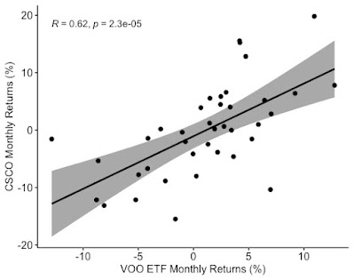
Linear Regression of Monthly Returns of Cisco Systems and the Vanguard S&P 500 Index ETF

Here is the graph of monthly returns of Cisco Systems (CSCO) plotted against Vanguard S&P 500 Index ETF (VOO):

Exhibit 1: Monthly Returns of Cisco Systems and Vanguard S&P 500 Index ETF [June 2019 -  August 2022]

Monthly Returns of the Vanguard S&P 500 Index ETF and Cisco Systems Inc.

(Source: RStudio, ggplot, Data Provided by IEX Cloud)

Results of the linear regression of monthly returns of Cisco Systems against Vanguard S&P 500 Index ETF:

VOOandCSCO <- read_excel("/CSCO_VOO_LM_September_2022.xlsx", sheet = "Sheet1")

lmCSCOVOO = lm(CSCO_Monthly_Return~VOO_Monthly_Return, data = VOOandCSCO)

summary(lmCSCOVOO)

Call:

lm(formula = CSCO_Monthly_Return ~ VOO_Monthly_Return, data = VOOandCSCO)

Residuals:

      Min        1Q    Median        3Q       Max 

-0.156924 -0.031998 -0.008248  0.038045  0.127839 

Coefficients:

                   Estimate Std. Error t value Pr(>|t|)    

(Intercept)        -0.01062    0.01049  -1.012    0.318    

VOO_Monthly_Return  0.91708    0.18946   4.841 2.31e-05 ***

---

Signif. codes:  0 ‘***’ 0.001 ‘**’ 0.01 ‘*’ 0.05 ‘.’ 0.1 ‘ ’ 1

Residual standard error: 0.06426 on 37 degrees of freedom

Multiple R-squared:  0.3877, Adjusted R-squared:  0.3712 

F-statistic: 23.43 on 1 and 37 DF,  p-value: 2.306e-05

The slope of the regression corresponds to the beta of the stock. In this case, Cisco Systems has a beta of 0.91. 

The adjusted R-squared is 0.37. About 37% of Cisco's monthly return is explained by the returns of the S&P 500 index.  

Cisco Systems cannot protect a portfolio against market volatility since it has a beta value close to 1. Cisco's stock will almost entirely reflect the volatility in the market.      

 

Linear Regression of Monthly Returns of Colgate-Palmolive against Vanguard S&P 500 Index ETF

Here is the graph of monthly returns of Colgate-Palmolive (CL) plotted against Vanguard S&P 500 Index ETF (VOO):

Exhibit 1: Monthly Returns of Colgate-Palmolive and Vanguard S&P 500 Index ETF [June 2019 -  August 2022]

(Source: RStudio, ggplot, Data Provided by IEX Cloud)

Results of the linear regression of monthly returns of Colgate-Palmolive against Vanguard S&P 500 Index ETF:

> VOOandCL <- read_excel("/CL_VOO_LM_September_2022.xlsx", sheet = "Sheet1")

> lmCLVOO = lm(CL_Monthly_Return~VOO_Monthly_Return, data = VOOandCL)

> summary(lmCLVOO)

Call:

lm(formula = CL_Monthly_Return ~ VOO_Monthly_Return, data = VOOandCL)

Residuals:

      Min        1Q    Median        3Q       Max 

-0.084505 -0.025451  0.002263  0.028820  0.122836 

Coefficients:

                    Estimate Std. Error t value Pr(>|t|)   

(Intercept)        0.0002236  0.0067940   0.033  0.97392   

VOO_Monthly_Return 0.3471172  0.1226847   2.829  0.00749 **

---

Signif. codes:  0 ‘***’ 0.001 ‘**’ 0.01 ‘*’ 0.05 ‘.’ 0.1 ‘ ’ 1

Residual standard error: 0.04161 on 37 degrees of freedom

Multiple R-squared:  0.1779, Adjusted R-squared:  0.1557 

F-statistic: 8.005 on 1 and 37 DF,  p-value: 0.007492

The slope of the regression corresponds to the beta of the stock. In this case, Colgate-Palmolive has a beta of 0.34. 

The adjusted R-squared is 0.15. About 15% of Colgate-Palmolive's return is explained by the returns of the S&P 500 index.  

Colgate-Palmolive can protect a portfolio against market volatility since it has a beta value substantially less than 1.    

 

Linear Regression of Monthly Returns of Lennox International against Vanguard S&P 500 Index ETF

Here is the graph of monthly returns of Lennox International (LII) plotted against Vanguard S&P 500 Index ETF (VOO):

Exhibit 1: Monthly Returns of Lennox International and Vanguard S&P 500 Index ETF [June 2019 -  August 2022 

(Source: RStudio, ggplot, Data Provided by IEX Cloud)

Results of the linear regression of monthly returns of Lennox International against Vanguard S&P 500 Index ETF:

VOOandLII <- read_excel("/LII_VOO_LM_September_2022.xlsx", sheet = "Sheet1")

lmLIIVOO = lm(LII_Monthly_Return~VOO_Monthly_Return, data = VOOandLII)

> summary(lmLIIVOO)

Call:

lm(formula = LII_Monthly_Return ~ VOO_Monthly_Return, data = VOOandLII)

Residuals:

      Min        1Q    Median        3Q       Max 

-0.090246 -0.052733 -0.001907  0.040310  0.108446 

Coefficients:

                    Estimate Std. Error t value Pr(>|t|)    

(Intercept)        -0.010082   0.009416  -1.071    0.291    

VOO_Monthly_Return  0.995050   0.170040   5.852 9.97e-07 ***

---

Signif. codes:  0 ‘***’ 0.001 ‘**’ 0.01 ‘*’ 0.05 ‘.’ 0.1 ‘ ’ 1

Residual standard error: 0.05767 on 37 degrees of freedom

Multiple R-squared:  0.4807, Adjusted R-squared:  0.4666 

F-statistic: 34.24 on 1 and 37 DF,  p-value: 9.966e-07

The slope of the regression corresponds to the beta of the stock. In this case, Lennox International has a beta of 0.995. Lennox's beta is close to the S&P 500 beta, so Lennox will move in line with the market.  

The adjusted R-squared is 0.46. About 46% of Lennox's return is explained by the returns of the S&P 500 index.  

Invest in an Equal-Weight ETF in these Turbulent Times.

The S&P 500 index is market-capitalization-weighted. The weighting by market cap means the companies with the largest market capitalization (Market capitalization = Number of shares outstanding x Share Price) get the highest weight. Last year, this method for calculating the index made the five largest companies by market cap account for 23% of the index. That is just 5 out of the 500 companies accounting for about a quarter of the market capitalization. These five companies were: Apple, Microsoft, Alphabet (Google), Amazon, and Facebook (Meta). When the share price of these companies starts underperforming, the market takes a huge tumble. We can see that happening now. The S&P 500 index (VOO) is down about 9.72% (pre-market on January 28), while the S&P 500 equal-weighted ETF (RSP) is down 7.48% (See Exhibit 1: Invesco Equal-Weight ETF Beats Vanguard S&P 500 Market-Cap Weighted ETF). That is a difference in the performance of 224 basis points. In essence, the equal-weight ETF outperformed the market-cap ETF. The dividend yield is about the same for both ETFs. The Invesco Equal-Weight ETF charges a higher expense ratio than the Vanguard S&P 500 ETF. Invesco charges 20 basis points (bps) or 0.2%, while the Vanguard S&P 500 ETF (VOO) charges three bps or 0.03%. Invesco charges 7x more than the Vanguard ETF. Even after deducting the extra expense of investing in the Invesco ETF, it comes ahead in performance by over 200 bps.  

The era of big-tech is coming to an end due to more regulation and their size inhibiting growth. At least for now, Apple seems to be bucking the trend after reporting blockbuster results yesterday. Interest rates are also rising, putting pressure on valuation because future earnings will be discounted at a higher interest rate. It may be good to have a position in the Invesco Equal-Weight ETF (RSP) during these times. 

     Exhibit 1: Invesco Equal-Weight ETF Beats Vanguard S&P 500 Market-Cap Weighted ETF

(Source: Seeking Alpha)

Also, there may be other equal-weight ETFs in the market. I am aware of Invesco's ETF, so I have invested in it. I am not endorsing the Invesco ETF.